Generalized mosaic plot with formula-based variable nesting

Usage

geom_marimekko(
  mapping = NULL,
  data = NULL,
  formula = NULL,
  gap = 0.01,
  gap_x = NULL,
  gap_y = NULL,
  colour = NULL,
  alpha = 0.9,
  show_percentages = FALSE,
  na.rm = FALSE,
  show.legend = NA,
  inherit.aes = TRUE,
  ...
)

Arguments

mapping

Aesthetic mapping. Optionally accepts fill and weight for pre-aggregated data. If fill is not specified, it defaults to the last variable in the formula. The fill variable controls tile colour and does not need to appear in the formula.

data

A data frame.

formula

A one-sided formula specifying the mosaic hierarchy. See the sections above for a detailed explanation.

Quick reference:

~ a | b — h(a), v(b). Standard mosaic.
~ a | b | c — h(a), v(b), h(c). Alternating mosaic.
~ a + b | c — h(a), h(b), v(c). Double decker.
~ a | b + c — h(a), v(b), v(c). Multiple vertical variables.

gap

Numeric. Gap between tiles as fraction of plot area. Default 0.01.

gap_x

Numeric. Horizontal gap override. Default NULL (uses gap).

gap_y

Numeric. Vertical gap override. Default NULL (uses gap).

colour

Tile border colour. Default NULL (no border). Can also be mapped via aes(colour = variable).

alpha

Tile transparency. Default 0.9.

show_percentages

Logical. If TRUE, appends marginal percentage to each x-axis label. Default FALSE.

na.rm

Logical. Remove missing values. Default FALSE.

show.legend

Logical. Show legend. Default NA.

inherit.aes

Logical. Inherit aesthetics from ggplot(). Default TRUE.

...

Additional arguments passed to the layer.

Value

A list of ggplot2 layers (geom + axis scales).

How the formula works

The formula uses two operators to encode the full partitioning hierarchy in a single expression:

| (pipe): Separates nesting levels. Each | switches the splitting direction, alternating horizontal, vertical, horizontal, vertical, and so on. The first variable (or group) listed is the outermost split — it partitions the entire plot area. Each subsequent level partitions the tiles created by the previous level.
+ (plus): Groups variables at the same nesting level. All variables joined by + share the same splitting direction and are applied sequentially within that level. The first + variable partitions the current tiles, then the second + variable further subdivides those tiles, still in the same direction.

Reading order — outermost to innermost

The formula is read left to right, from the coarsest (outermost) partition to the finest (innermost):

~ a | b: First split the plot horizontally by a (columns whose widths reflect marginal proportions of a). Then, within each column, split vertically by b (rows whose heights reflect conditional proportions of b given a). This is the classic two-variable marimekko / mosaic plot.
~ a | b | c: Horizontal by a, then vertical by b, then horizontal again by c. Three levels of nesting with alternating directions (h \(\to\) v \(\to\) h).
~ a + b | c: Horizontal by a, then horizontal again by b (same direction because + groups them), then vertical by c. This is the double decker pattern — all horizontal splits first, with a single vertical split at the end.
~ a | b + c: Horizontal by a, then vertical by b, then vertical again by c. Two vertical variables nested within each column.

Computed variables

The stat computes the following variables that can be accessed with ggplot2::after_stat():

.proportion: Conditional proportion of the tile within its immediate parent. For a formula ~ a | b, this is the proportion of b within each level of a, i.e. \(P(b \mid a)\). Values sum to 1 within each parent tile. Useful for mapping to alpha to fade tiles by their local share: aes(alpha = after_stat(.proportion)).
.marginal: Joint (marginal) proportion of the tile relative to the whole dataset, i.e. \(n_\text{cell} / N\). Values sum to 1 across all tiles. Used internally for x-axis percentage labels when show_percentages = TRUE, and can be mapped to aesthetics to emphasise cells by overall frequency.
.residuals: Pearson residual measuring departure from statistical independence between the horizontal and vertical variable groups. Computed as \((O - E) / \sqrt{E}\), where \(O\) is the observed cell count and \(E\) is the count expected under independence. Positive values indicate the cell is more frequent than expected; negative values indicate less frequent. When only one direction (all horizontal or all vertical) is present, .residuals is set to 0. Map to alpha or fill to highlight deviations: aes(alpha = after_stat(abs(.residuals))).

Examples

library(ggplot2)

titanic <- as.data.frame(Titanic)

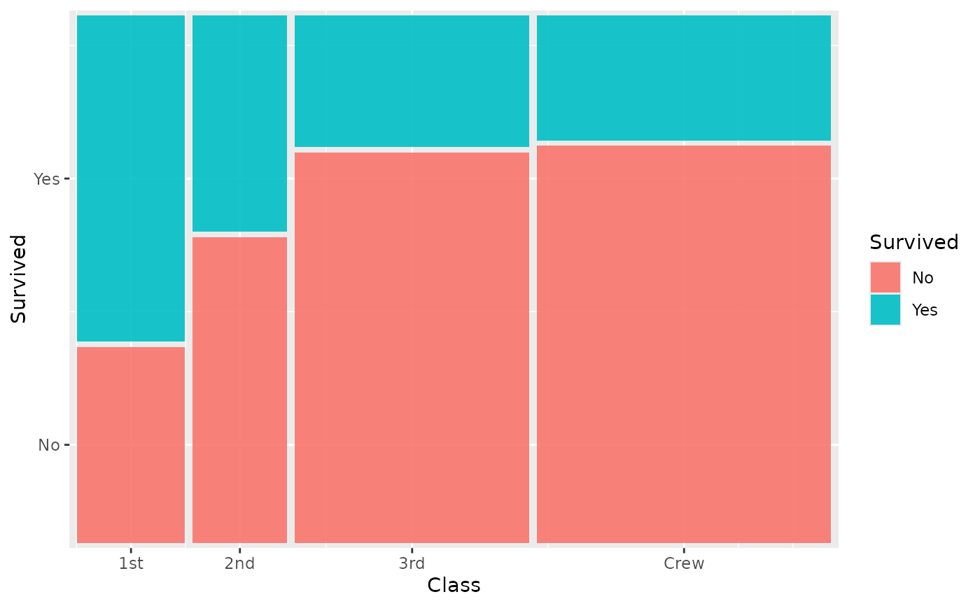
# 2-variable mosaic
ggplot(titanic) +
  geom_marimekko(
    aes(fill = Survived, weight = Freq),
    formula = ~ Class | Survived
  )


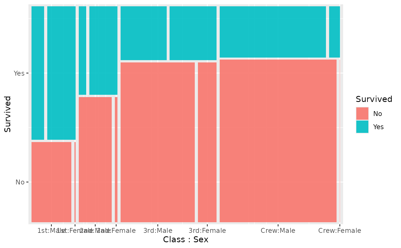
# 3-variable mosaic (h -> v -> h)
ggplot(titanic) +
  geom_marimekko(
    aes(fill = Survived, weight = Freq),
    formula = ~ Class | Survived | Sex
  )


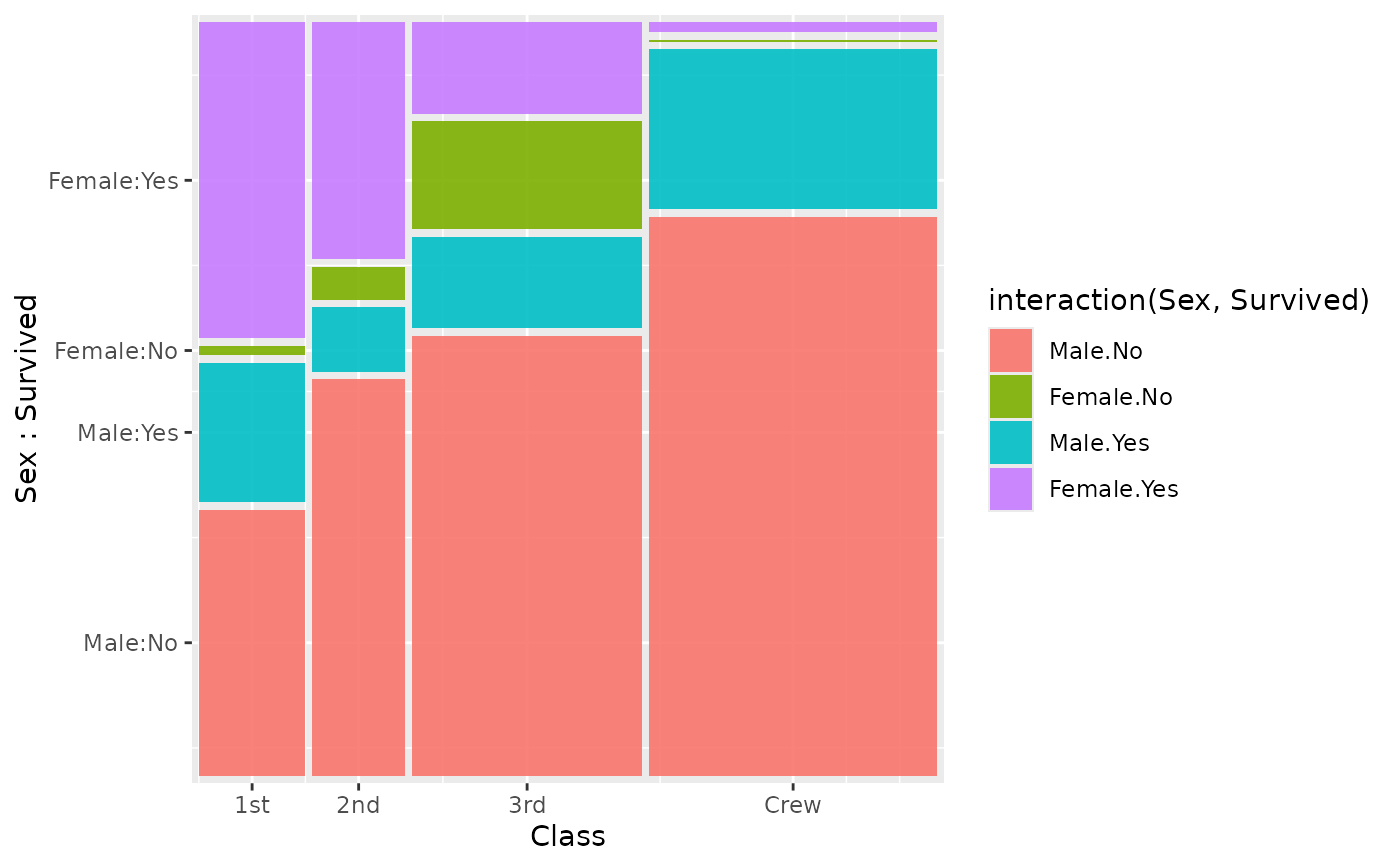
# Multi-variable fill with interaction()
ggplot(titanic) +
  geom_marimekko(
    aes(fill = interaction(Sex, Survived), weight = Freq),
    formula = ~ Class | Sex + Survived
  )


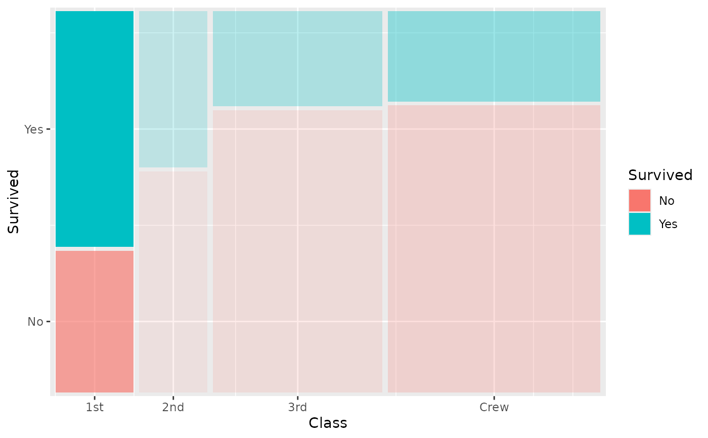
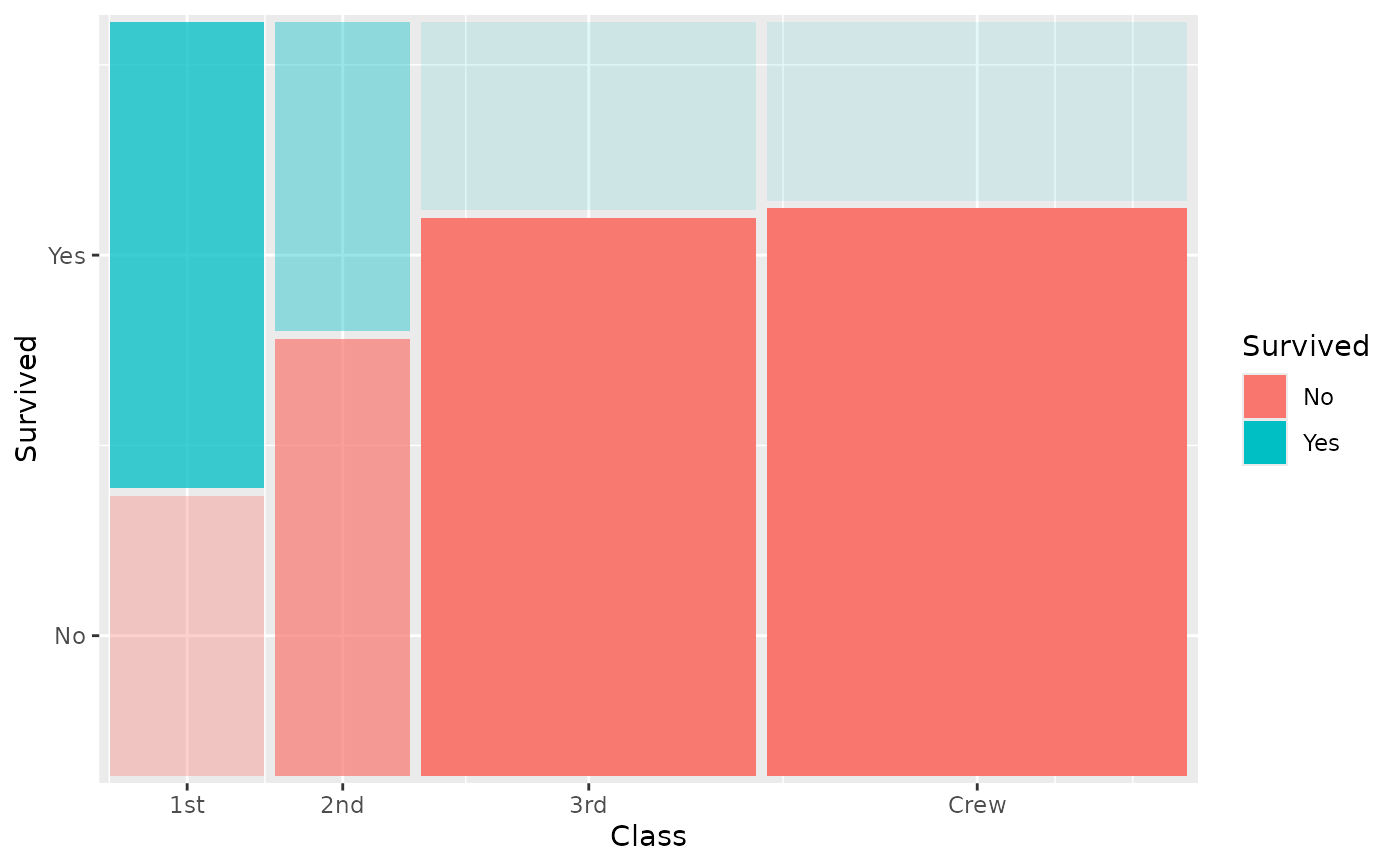
# Fade tiles by conditional proportion
ggplot(titanic) +
  geom_marimekko(
    aes(fill = Survived, alpha = after_stat(.proportion), weight = Freq),
    formula = ~ Class | Survived
  ) +
  guides(alpha = "none")


# Highlight cells that deviate from independence
ggplot(titanic) +
  geom_marimekko(
    aes(fill = Survived, alpha = after_stat(abs(.residuals)), weight = Freq),
    formula = ~ Class | Survived
  ) +
  guides(alpha = "none")