Migrating from ggmosaic to marimekko

Why migrate?

ggmosaic was archived from CRAN on 2025-11-10 due to uncorrected issues. Key problems included reliance on internal ggplot2 APIs that broke on updates and a dependency on deprecated tidyr functions.

marimekko is a from-scratch replacement that uses only public ggplot2 APIs, depends only on ggplot2 and rlang, and follows standard ggplot2 aesthetic conventions.

The examples below are adapted from Jeppson & Hofmann (2023), showing each ggmosaic pattern and its marimekko equivalent.

Function mapping

ggmosaic	marimekko	Notes
geom_mosaic()	geom_marimekko()	Standard aes(), no product()
geom_mosaic_text()	geom_marimekko_text()
theme_mosaic()	theme_marimekko()
scale_x_productlist()	not needed	Axis labels are automatic; use show_percentages = TRUE in geom_marimekko()
scale_y_productlist()	not needed	Axis labels are automatic
product()	not needed	Use formula = ~ a \| b
—	geom_marimekko_label()	New: text with background box
—	fortify_marimekko()	New: extract tile data as data frame

Side-by-side examples

The ggmosaic paper (Jeppson & Hofmann, 2023, The R Journal 14(4)) uses the fly dataset from ggmosaic and the built-in Titanic dataset. Since ggmosaic is no longer on CRAN, we recreate the fly-based examples using Titanic and HairEyeColor — both built-in R datasets that need no extra packages.

One dimensional — spine plot and bar chart

The paper starts with single-variable plots showing different divider types (Figure 1 in Jeppson & Hofmann, 2023):

# ggmosaic — spine plot (one variable, default divider)
ggplot(data = titanic) +
  geom_mosaic(aes(x = product(Class), fill = Class, weight = Freq))

# marimekko — one variable
ggplot(titanic) +
  geom_marimekko(aes(fill = Class, weight = Freq), formula = ~Class) +
  theme_marimekko() +
  labs(title = "One variable: f(Class)")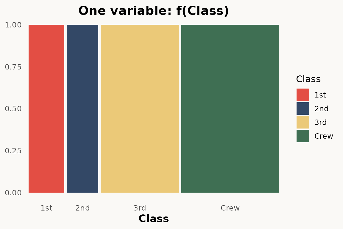

# ggmosaic — bar chart (one variable, hbar divider)
ggplot(data = titanic) +
  geom_mosaic(
    aes(x = product(Class), fill = Class, weight = Freq),
    divider = "hbar"
  )

# ggplot — barchart
# todo: needs percentage y scale
ggplot(titanic) +
  geom_bar(aes(Class, weight = Freq, fill = Class)) +
  theme_marimekko() +
  labs(title = "One variable: f(Class)")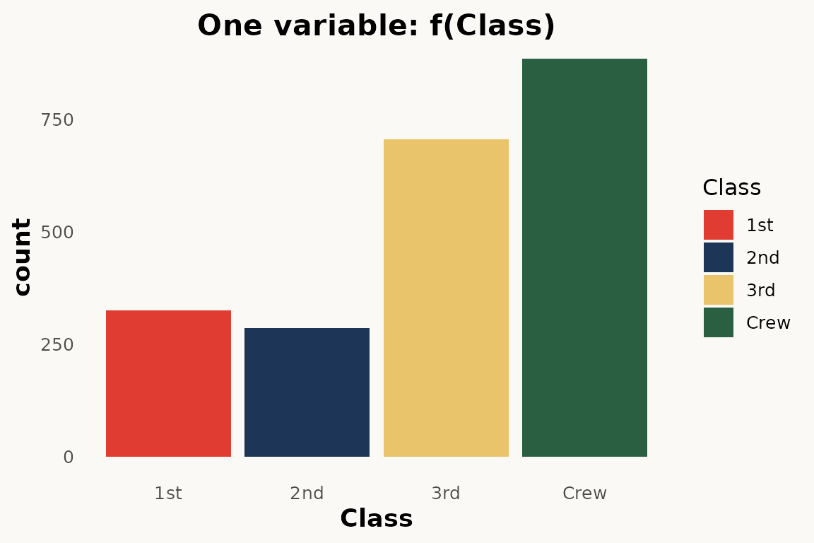

The main difference: no product() wrapper — use formula = ~ Var instead. marimekko does not have a divider argument; it always produces vertical columns with horizontal stacking.

Two dimensional — mosaic plot and stacked bar chart

The paper shows two-dimensional mosaic plots where variable order in product() controls the partitioning hierarchy (Figure 2):

# ggmosaic — two variables
ggplot(data = titanic) +
  geom_mosaic(aes(
    x = product(Class),
    fill = Survived,
    weight = Freq
  ))

# marimekko — two variables via formula
ggplot(titanic) +
  geom_marimekko(aes(fill = Survived, weight = Freq),
    formula = ~ Class | Survived
  ) +
  theme_marimekko() +
  labs(title = "Two variables: f(Survived | Class) f(Class)")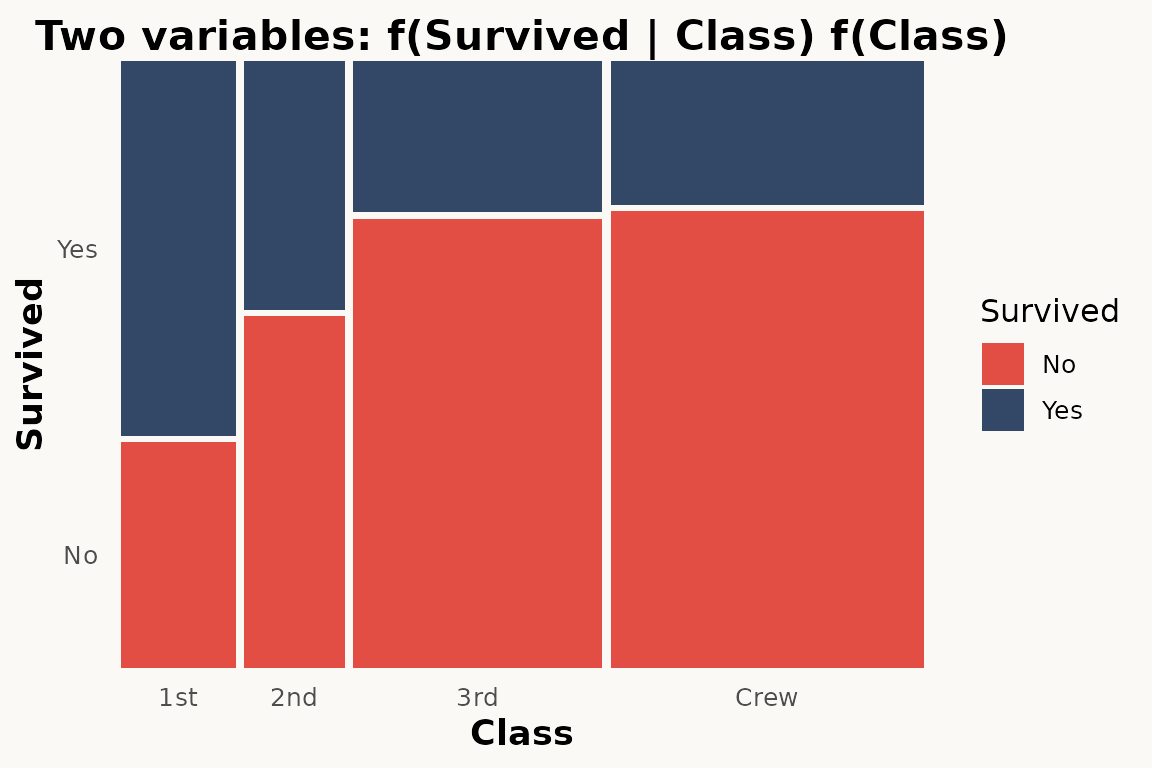

Three dimensional

The paper shows two-dimensional mosaic plots where variable order in product() controls the partitioning hierarchy (Figure 3):

# ggmosaic — double-decker variables
ggplot(data = titanic) +
  geom_mosaic(aes(
    x = product(Survived, Class, Sex),
    fill = Survived,
    weight = Freq,
  ), divider = ddecker())

# marimekko — three variables via formula
ggplot(titanic) +
  geom_marimekko(aes(fill = Survived, weight = Freq),
    formula = ~ Sex + Class | Survived
  ) +
  theme_marimekko() +
  labs(title = "Three variables: f(Survived | Class, Sex)")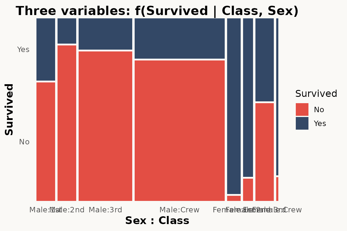

Three variables — nested mosaic

The paper demonstrates three-variable mosaics where a third variable adds another level of partitioning (Figure 4):

# ggmosaic — three variables via product()
ggplot(data = titanic) +
  geom_mosaic(aes(
    x = product(Sex, Survived, Class),
    fill = Survived,
    weight = Freq
  ))

# marimekko — three variables via formula
ggplot(titanic) +
  geom_marimekko(aes(fill = Survived, weight = Freq),
    formula = ~ Class | Survived | Sex
  ) +
  theme_marimekko() +
  labs(title = "Three variables: Class / Sex / Survived")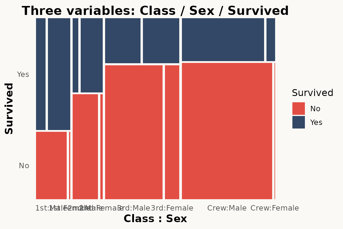

Conditioning with conds

The paper shows how conds creates conditional distributions (Section 3.2):

# ggmosaic — conditioning
ggplot(data = titanic) +
  geom_mosaic(aes(
    x = product(Class),
    fill = Survived,
    weight = Freq,
    conds = product(Sex)
  ))

marimekko does not have a conds aesthetic. Use facet_wrap() instead:

# marimekko — conditioning via faceting
ggplot(titanic) +
  geom_marimekko(aes(fill = Survived, weight = Freq),
    formula = ~ Class | Survived
  ) +
  facet_wrap(~Sex) +
  theme_marimekko() +
  labs(title = "f(Survived | Class) conditioned on Sex")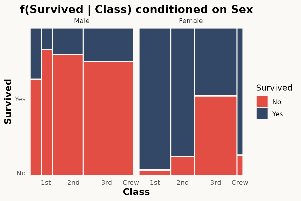

Faceting

The paper demonstrates facet_grid() as an alternative to conditioning (Section 3.3):

# ggmosaic — faceting
ggplot(data = titanic) +
  geom_mosaic(aes(
    x = product(Class), fill = Survived, weight = Freq
  )) +
  facet_grid(~Sex)

# marimekko — faceting works the same way
ggplot(titanic) +
  geom_marimekko(aes(fill = Survived, weight = Freq),
    formula = ~ Class | Survived
  ) +
  facet_wrap(~Sex) +
  theme_marimekko() +
  labs(title = "Mosaic faceted by Sex")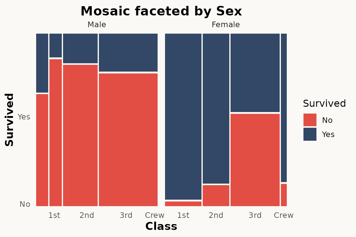

Divider types and standardize

The paper describes four fundamental partition types: hspine, vspine, hbar, and vbar (Section 4, Figure 5). These are combined to produce spine plots, stacked bar charts, mosaic plots, and double decker plots.

marimekko simplifies this — geom_marimekko() always starts with horizontal splits and alternates direction with each | in the formula. Use coord_flip() if you need vertical-first orientation.

For equal-width columns (spine-plot style), standardize = TRUE is available in geom_marimekko_text() and fortify_marimekko().

# ggmosaic — spine plot via divider
ggplot(titanic) +
  geom_mosaic(aes(x = product(Class), fill = Survived, weight = Freq),
    divider = c("vspine", "hspine")
  )

# marimekko — proportional-width columns (default)
ggplot(titanic) +
  geom_marimekko(aes(fill = Survived, weight = Freq),
    formula = ~ Class | Survived
  ) +
  theme_marimekko() +
  labs(title = "Mosaic plot (proportional-width columns)")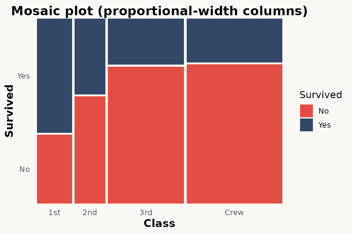

Offset / spacing

The paper shows how offset controls gaps between tiles (Section 5):

# ggmosaic — single offset parameter
ggplot(data = titanic) +
  geom_mosaic(aes(
    x = product(Class), fill = Survived, weight = Freq
  ), offset = 0.02)

marimekko provides independent gap_x and gap_y parameters:

# marimekko — no gaps
ggplot(titanic) +
  geom_marimekko(aes(fill = Survived, weight = Freq),
    formula = ~ Class | Survived, gap_x = 0.02, gap_y = 0.02
  ) +
  theme_marimekko() +
  labs(title = "No gaps")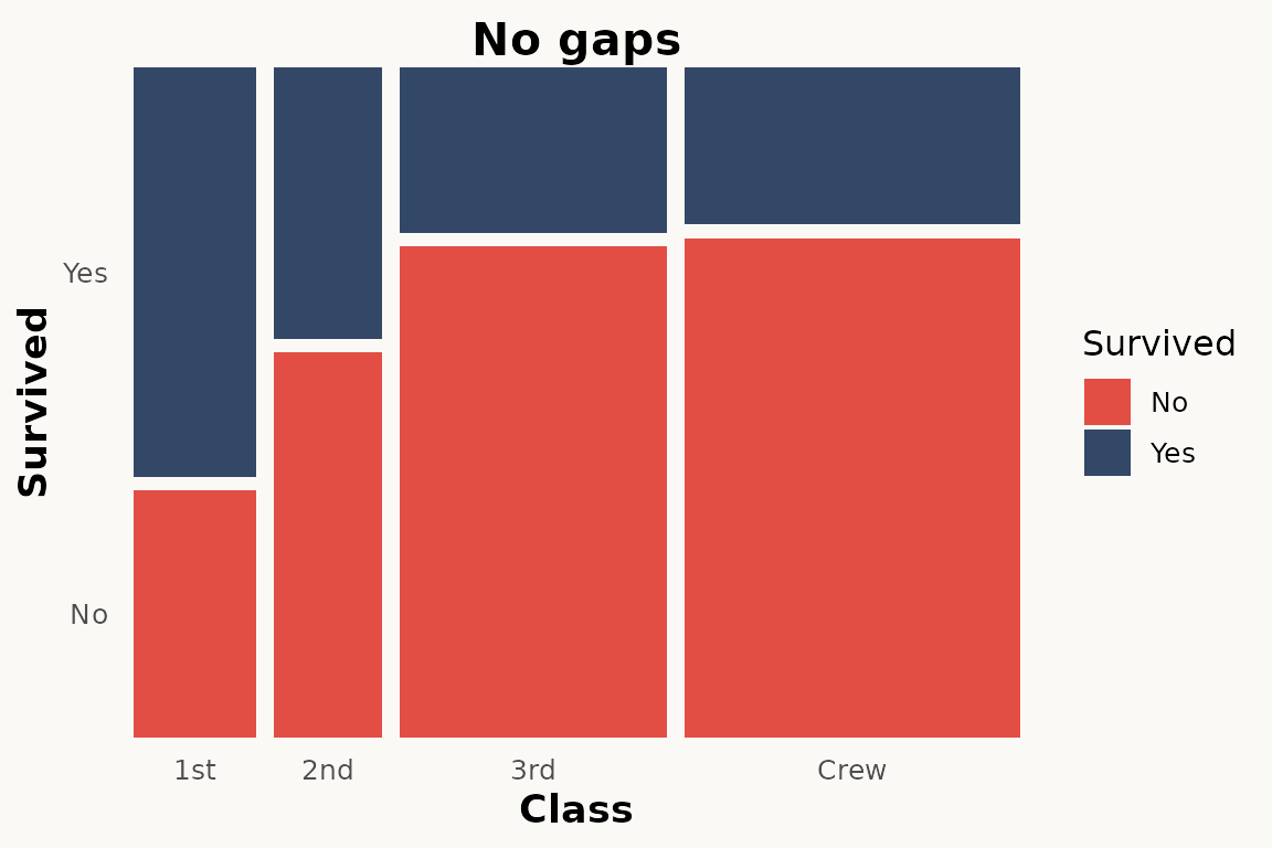

Text labels

The paper shows geom_mosaic_text() for adding labels (Section 7):

# ggmosaic — automatic text labels
ggplot(titanic) +
  geom_mosaic(aes(x = product(Class), fill = Survived, weight = Freq)) +
  geom_mosaic_text(aes(x = product(Class), fill = Survived, weight = Freq))

# marimekko — automatic tile positions, only label needed
ggplot(titanic) +
  geom_marimekko(aes(fill = Survived, weight = Freq),
    formula = ~ Class | Survived
  ) +
  geom_marimekko_text(aes(
    label = after_stat(paste(Class, Survived, sep = "\n"))
  )) +
  theme_marimekko()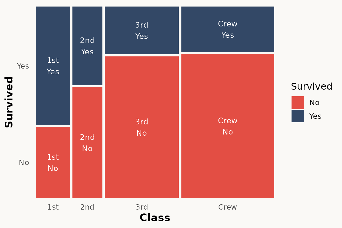

geom_marimekko_text() reads tile positions from the preceding geom_marimekko() layer — only the label aesthetic is needed. Use after_stat() for computed variables like weight (count), .proportion, or the original variable columns.

Axis labels and percentages

The paper uses scale_x_productlist() for axis labels:

# ggmosaic
ggplot(titanic) +
  geom_mosaic(aes(x = product(Class), fill = Survived, weight = Freq)) +
  scale_x_productlist()

# marimekko — with optional marginal percentages
ggplot(titanic) +
  geom_marimekko(aes(fill = Survived, weight = Freq),
    formula = ~ Class | Survived,
    show_percentages = TRUE
  ) +
  theme_marimekko()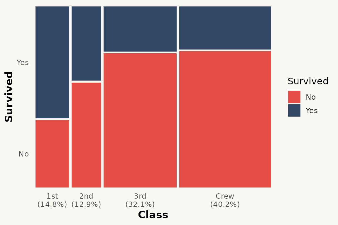

HairEyeColor — a larger example

The paper uses multi-variable examples to show how mosaic plots reveal associations. Here we use the built-in HairEyeColor dataset:

ggplot(hair) +
  geom_marimekko(aes(fill = Eye, weight = Freq),
    formula = ~ Hair | Eye,
    show_percentages = TRUE
  ) +
  theme_marimekko() +
  labs(title = "Hair color vs Eye color")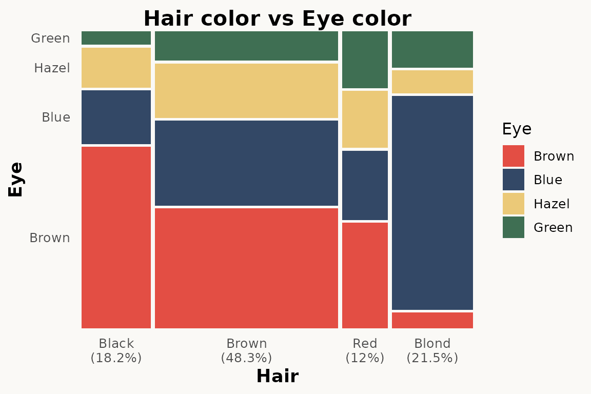

Three-variable version with Sex:

ggplot(hair) +
  geom_marimekko(aes(fill = Eye, weight = Freq),
    formula = ~ Hair | Sex | Eye
  ) +
  theme_marimekko() +
  labs(title = "Hair / Sex / Eye")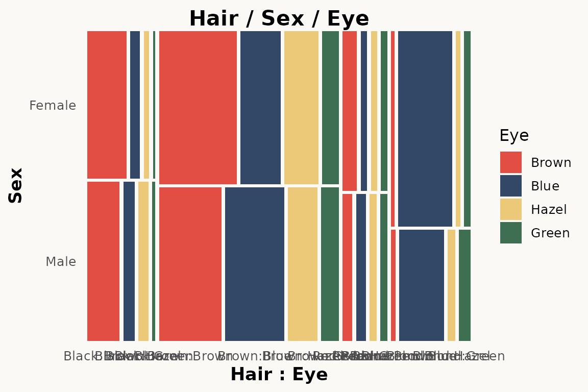

Key differences to be aware of

1. No product() wrapper

ggmosaic required wrapping variables in product(). marimekko uses a formula-based API:

• formula = ~ a | b — specifies variable hierarchy (| alternates direction, + groups)
• fill — tile colour (defaults to last formula variable)
• weight — observation weights / counts

2. Automatic axis labels

ggmosaic handled axis labels internally. marimekko also adds axis labels automatically via geom_marimekko(). Use show_percentages = TRUE in geom_marimekko() to append marginal percentages to the x-axis labels.

3. No divider argument

ggmosaic used divider = c("vspine", "hspine", ...) to control partitioning direction. marimekko encodes direction in the formula — | alternates between horizontal and vertical, always starting horizontal. Use coord_flip() for vertical-first orientation.

4. inherit.aes defaults to TRUE

ggmosaic set inherit.aes = FALSE by default, requiring you to repeat aesthetics in every layer. marimekko follows ggplot2 convention — inherit.aes = TRUE — so aesthetics set in ggplot(aes(...)) are inherited.

5. Text labels need explicit label aesthetic

geom_marimekko_text() requires label = after_stat(weight) or similar. ggmosaic’s geom_mosaic_text() auto-generated labels.

plotly support

marimekko plots work with plotly::ggplotly() out of the box — simply pass your plot object and get an interactive version:

library(plotly)

p <- ggplot(titanic) +
  geom_marimekko(aes(fill = Survived, weight = Freq),
    formula = ~ Class | Survived
  )

ggplotly(p)

This also works with geom_marimekko_text(), geom_marimekko_label()

Search-and-replace checklist

For a quick mechanical migration, apply these replacements:

geom_mosaic(          →  geom_marimekko(
geom_mosaic_text(     →  geom_marimekko_text(
theme_mosaic(         →  theme_marimekko(
library(ggmosaic)     →  library(marimekko)

Then manually:

1. Remove all product() wrappers – add formula = ~ Var1 | Var2 instead
2. Remove conds aesthetic – use facet_wrap() or a multi-variable formula
3. Remove scale_x_productlist() / scale_y_productlist() – axis labels are now automatic
4. Remove divider = ... – direction is encoded in the formula
5. Replace offset = ... with gap / gap_x / gap_y
6. Add explicit label = after_stat(weight) to text layers
7. Set inherit.aes = FALSE only where deliberately needed
8. Move show_percentages = TRUE from scale to geom_marimekko(..., show_percentages = TRUE)

References

Jeppson, H. and Hofmann, H. (2023). Generalized Mosaic Plots in the ggplot2 Framework. The R Journal, 14(4), 50–73. doi:10.32614/RJ-2023-013